Spatial Denoising
Welcome to the spatial denoising tutorial.
In this tutorial, we will show you the effect of noise reduction by using
the spatial denoising algorithm implemented in dynsight (Related paper: Donkor et al., Martino et al.).
We will also explain another application of the Onion Clustering algorithm to explore different time resolutions for the classification (trajectory.Insight.get_onion_analysis()).
At the end of this tutorial, you will find links to download the full python scripts
and its relevant input files.
1. Computing TimeSOAP
As explained in the getting started tutorial, the first step is to load a trajectory into a trajectory.Trj object:
from pathlib import Path
from dynsight.trajectory import Trj

files_path = Path("source/_static/simulations")
trj = Trj.init_from_xtc(
    traj_file=files_path / "ice_water_ox.xtc",
    topo_file=files_path / "ice_water_ox.gro",
)
In this tutorial, we will use the descriptor TimeSOAP (Caruso et al.).
Before understanding what TimeSOAP is, we need to define the Smooth Overlap of Atomic Positions (SOAP) spectra (Bartók et al.).
The SOAP descriptor, is a structural descriptor that provides a high-dimensional representation of the local structure
around a particle by encoding the relative spatial arrangement of neighboring particles into
a smooth and continuous representation.
In this sense, the SOAP power spectrum serves as a descriptor of the degree of local order or disorder in the relative displacements of
the weights around a center (symmetry, distances, etc.). TimeSOAP is a time-dependent descriptor that, starting from the structural description of local environments provided by SOAP,
detects and tracks high-dimensional fluctuations over time in the SOAP spectra.
It captures local structural changes or transitions in the neighborhood of every unit.
To compute TimeSOAP, we first need to compute the SOAP spectra. In dynsight, we can use the trajectory.Trj.get_soap() method:
Warning
Consider that the computation of SOAP can be computationally expensive depending on the system size or the parameters used and can produce very large datasets.
It is recommended to tune the n_max or l_max parameter and speed up the calculation with n_jobs (according to the amount of CPU cores of your machine).
# Computing SOAP descriptor
soap = trj.get_soap(
    r_cut=10,
    n_max=8,
    l_max=8,
    n_jobs=4, # Adjust n_jobs according to your computer capabilities
)
The soap variable is a trajectory.Insight object that contains the computed SOAP spectra.
We can now use this dataset to obtain the TimeSOAP descriptor with the trajectory.Insight.get_timesoap() method:
# Computing TimeSOAP descriptor
_, tsoap = trj.get_timesoap(
    soap_insight=soap,
)
Alternatively, we can compute the SOAP and TimeSOAP descriptors in a single step by using the trajectory.Trj.get_timesoap() method directly:
soap, tsoap = trj.get_timesoap(
    r_cut=10,
    n_max=8,
    l_max=8,
    n_jobs=4
)
The tsoap and soap variables are the same trajectory.Insight objects computed above.
2. Onion Clustering analysis
As seen in the getting started tutorial, once we have computed the TimeSOAP descriptor,
we can perform the clustering analysis using the Onion Clustering method.
Given a delta_t window (in frames), Onion assigns each particle to the cluster (identified through a Kernel Density Estimation of the entire dataset) where it spends all the time.
Particles that cannot be assigned to a cluster are labeled as “unclassified fraction”.
Through the trajectory.Insight.get_onion_analysis() method, we can perform the Onion Clustering recursively for different time windows (delta_t).
# Performing Onion Clustering on the descriptor computed
tsoap.get_onion_analysis(
    delta_t_min=2,
    delta_t_num=20,
    fig1_path=files_path / "onion_analysis.png",
)
This will perform the Onion Clustering analysis for 20 time windows from 2 frames to the entire simulation length.
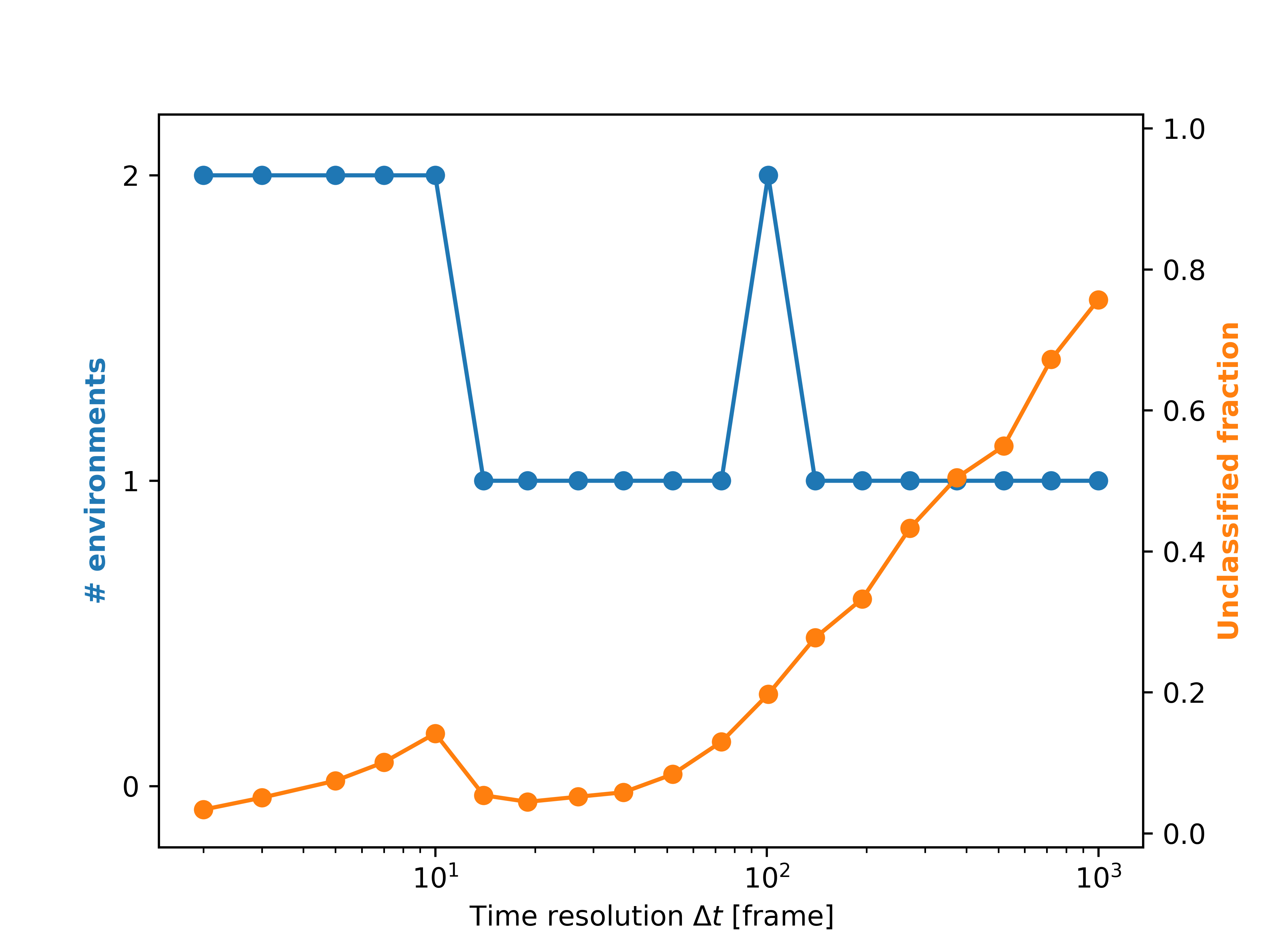
The plot shows how the number of clusters (blue line) and the unclassified fraction (orange line) change as a function of the time window.
3. Spatial Denoising
Nonetheless, the presence of noise in the trajectory can affect the quality of the clustering results.
To reduce the effect of noise, we can apply several denoising algorithms. Here, we will use the spatial denoising algorithm proposed by Donkor et al..
This algorithm works by averaging the descriptor values of neighboring particles within a cutoff radius r_cut.
As seen in the getting started tutorial for LENS, also TimeSOAP is computed for every pair of frames. Thus, the resulting dataset has shape
(n_particles, n_frames - 1). Consequently, we need to remove the last frame from the trajectory:
# Applying Spatial Denoising
sliced_trj = trj.with_slice(slice(0, -1, 1))
sp_denoised_tsoap = tsoap.spatial_average(
    trj=sliced_trj,
    r_cut=10,
    n_jobs=4, # Adjust n_jobs according to your computer capabilities
)
We can now repeat the Onion Clustering analysis on the denoised descriptor:
# Performing Onion Clustering on the descriptor computed
sp_denoised_tsoap.get_onion_analysis(
    delta_t_min=2,
    delta_t_num=20,
    fig1_path=files_path / "denoised_onion_analysis.png",
)
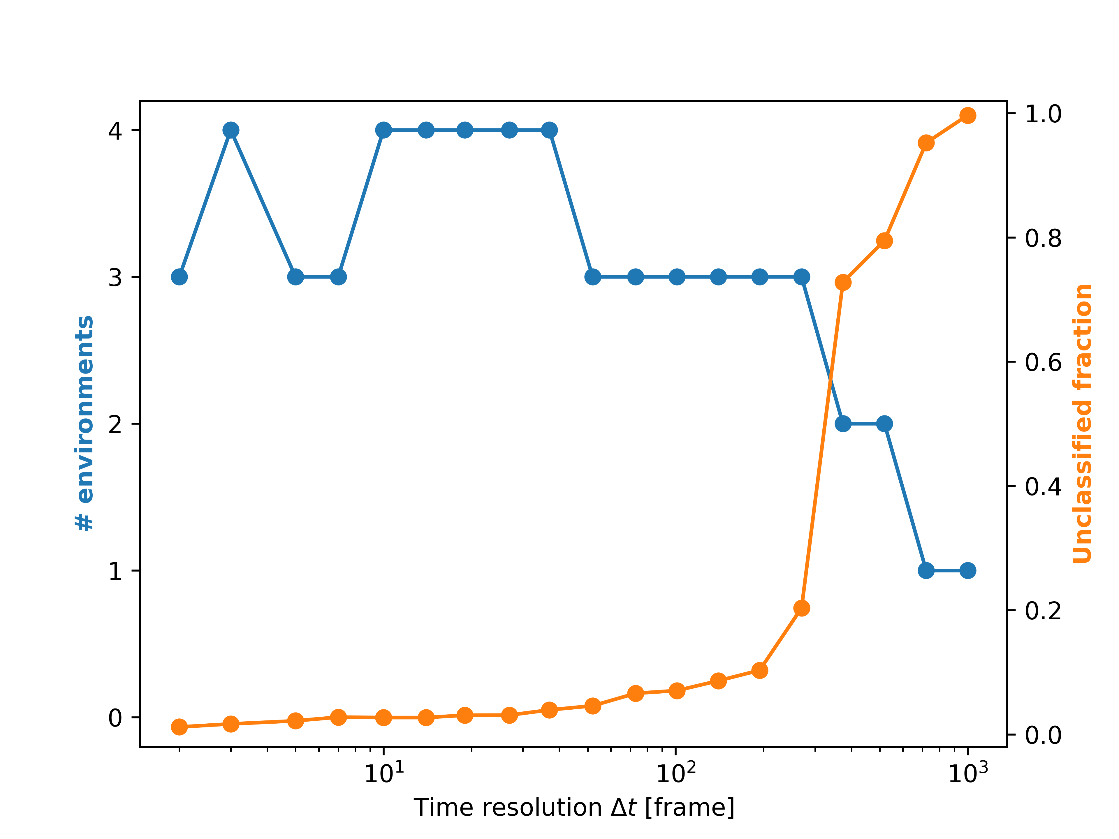
Comparing the two plots, we can see that the denoised descriptor leads to a higher number of clusters detected thanks to reduction of noise-related fluctuations in the data.
4. Visualization
Now we can select a specific time window and visualize the clustering results for both the raw and denoised descriptors. Here, we considered as the best
time window the one that corresponds to the highest number of clusters and longest delta_t (in this case, delta_t=37 frames).
This choice should guarantee that the clusters identified are stable for longer time.
single_point_onion = tsoap.get_onion_smooth(
    delta_t=37,
)
single_point_onion.dump_colored_trj(
    sliced_trj,
    files_path / "onion_trj.xyz",
)

denoised_single_point_onion = sp_denoised_tsoap.get_onion_smooth(
    delta_t=37,
)
denoised_single_point_onion.dump_colored_trj(
    sliced_trj,
    files_path / "onion_trj_denoised.xyz",
)
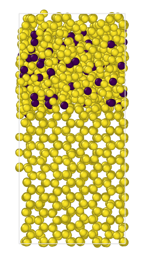
The resulting colored snapshots for the two descriptors (raw on the left, denoised on the right) are shown below:

Full scripts and input files
⬇️ Download the .gro file⬇️ Download the .xtc file
⬇️ Download Python Script