Cleaning Cluster Population

Sometimes, clusters obtained with Onion Clustering analysis can be very small. To better interpret the results, it can be useful to remove those ones by assigning them to the cluster of the unclassified particles. This is achieved through the class, data_processing.cleaning_cluster_population(), which assign the cluster under a certain population threshold to a specific cluster selected by the user.

At the end of every section, you will find links to download the full python scripts and its relevant input files.

As an example, we consider the ouput of the analysis computed in the spatial denoising tutorial. Briefly, we consider the denoised TimeSOAP descriptor that can be obtained from:

import numpy as np
from pathlib import Path
import dynsight
from dynsight.trajectory import Trj
from dynsight.data_processing import cleaning_cluster_population

files_path = Path("source/_static/simulations")
trj = Trj.init_from_xtc(
    traj_file=files_path / "ice_water_ox.xtc",
    topo_file=files_path / "ice_water_ox.gro",
)

_, tsoap = trj.get_timesoap(
    r_cut=10,
    n_max=8,
    l_max=8,
    n_jobs=4, # Adjust n_jobs according to your computer capabilities
)

sliced_trj = trj.with_slice(slice(0, -1, 1))
sp_denoised_tsoap = tsoap.spatial_average(
    trj=sliced_trj,
    r_cut=10,
    n_jobs=4, # Adjust n_jobs according to your computer capabilities
)

delta_t_list, n_clust, unclass_frac, labels = sp_denoised_tsoap.get_onion_analysis(
    delta_t_min=2,
    delta_t_num=20,
    fig1_path=files_path / "denoised_onion_analysis.png",
    fig2_path=files_path / "cluster_population.png",
)

For further details users should refer to spatial denoising tutorial.

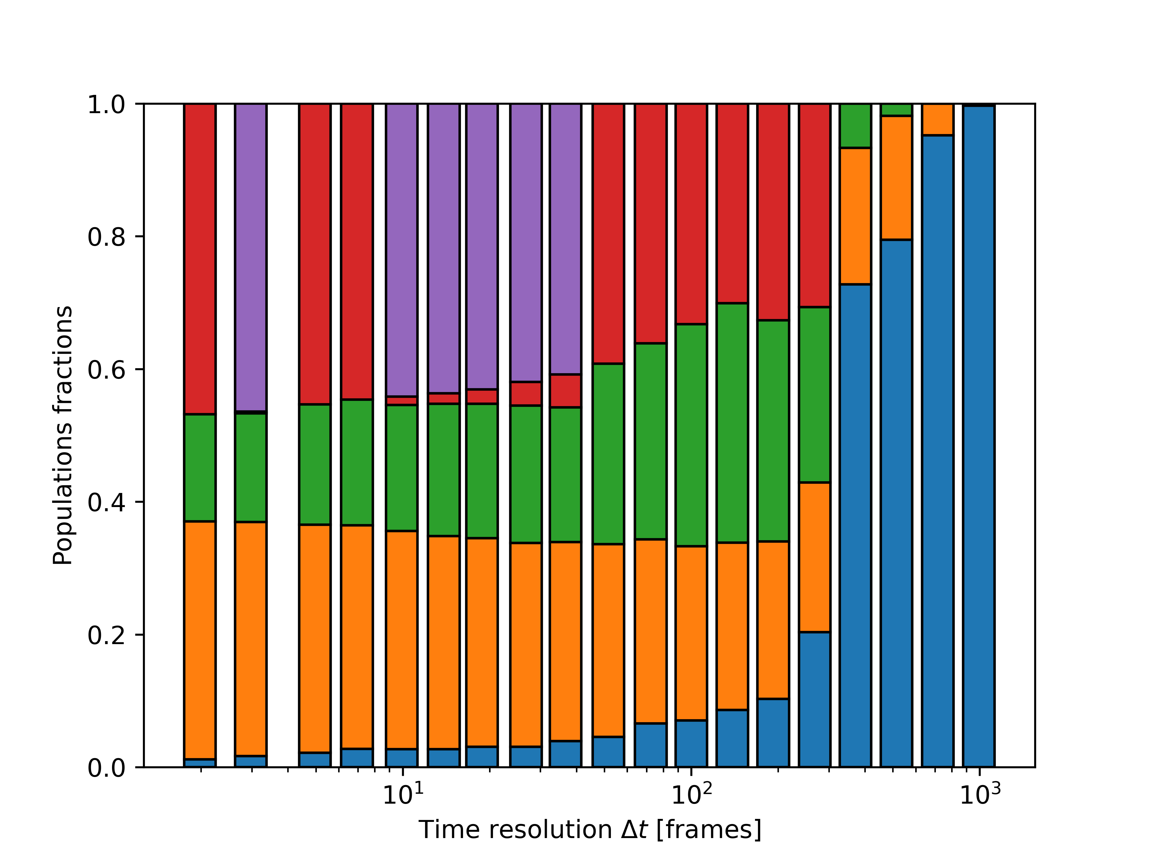
Figure cluster_population.png shows the population of every cluster, each color is a different cluster and blue refers to the unclassified fraction:

Before cleaning the cluster we have to save the output from the Onion analysis in an array:

onion_output = np.array([delta_t_list, n_clust, unclass_frac]).T

The small clusters can be removed and assigned to the unclassified fraction using the class data_processing.cleaning_cluster_population():

cleaned_labels = cleaning_cluster_population(labels, threshold=0.05, assigned_env=-1)

where cleaned_labels has the same dimensions as labels. Now we can reproduce the plot with the number of clusters and the unclassified fraction after re-organizing the data. In particular, onion.plot_smooth.plot_time_res_analysis(), which gives the plot that we want to obtain, requires and array with the list of the time windows, the number of clusters at every ∆t, and the unclassified fraction. Therefore, before plotting the graph, we need to create it by copying the list of time windows from the one given by the Onion analysis, and calculate the number of clusters and the unclassified fraction from the cleaned labels:

delta_t_list = onion_output[:, 0]  # Since unchanged, windows can be copied from above.

n_clust = np.zeros(delta_t_list.shape[0],dtype=np.int64)
unclass_frac = np.zeros(delta_t_list.shape[0])
for i in range(delta_t_list.shape[0]):
    n_clust[i] = np.unique(cleaned_labels[:, :, i]).size - 1
    unclass_frac[i] = np.sum(cleaned_labels[:, :, i] == -1) / np.size(cleaned_labels[:, :, i])

cleaned_onion_output = np.array([delta_t_list, n_clust, unclass_frac]).T

dynsight.onion.plot_smooth.plot_time_res_analysis("cleaned_onion_analysis.png", cleaned_onion_output)

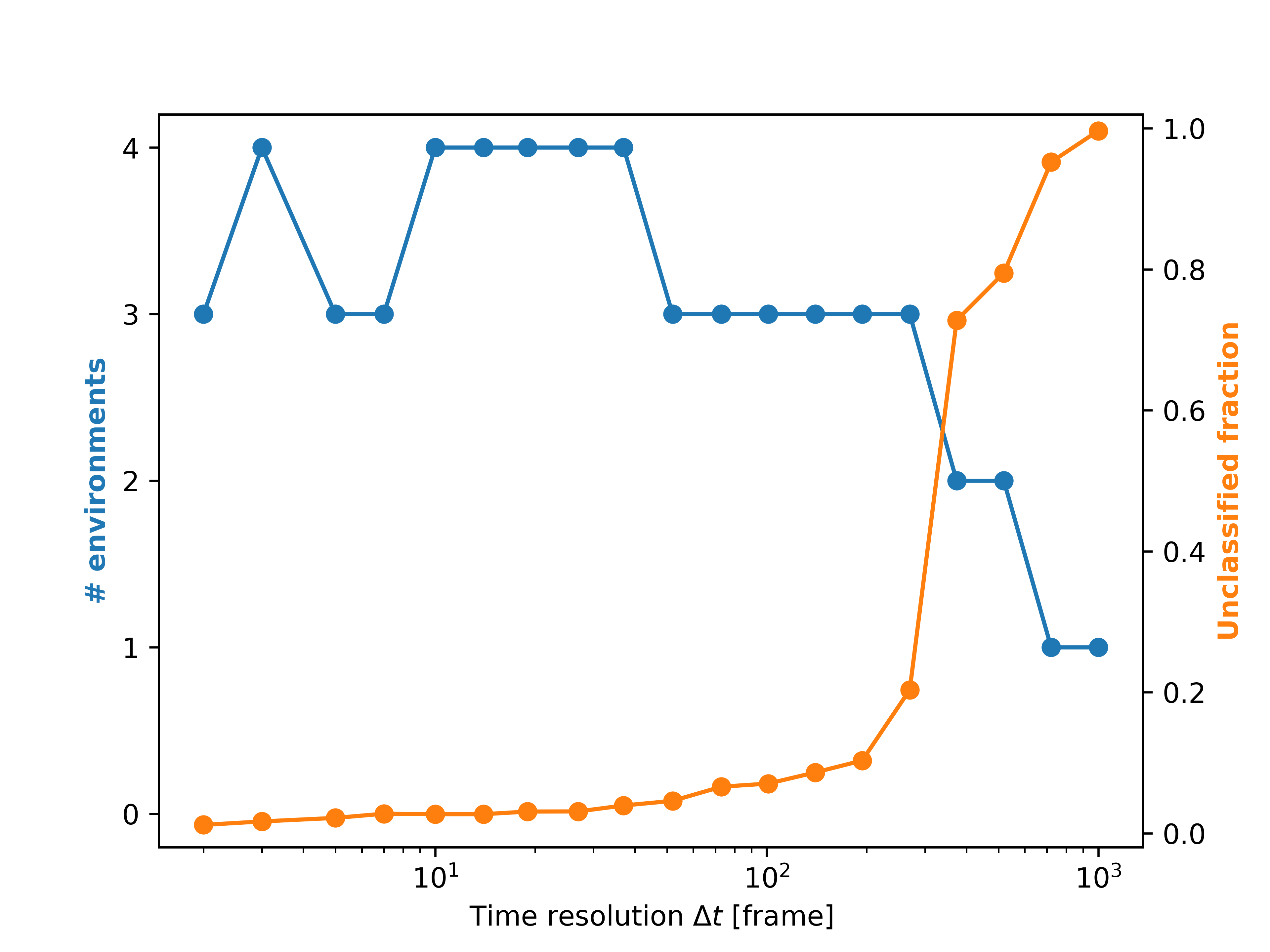
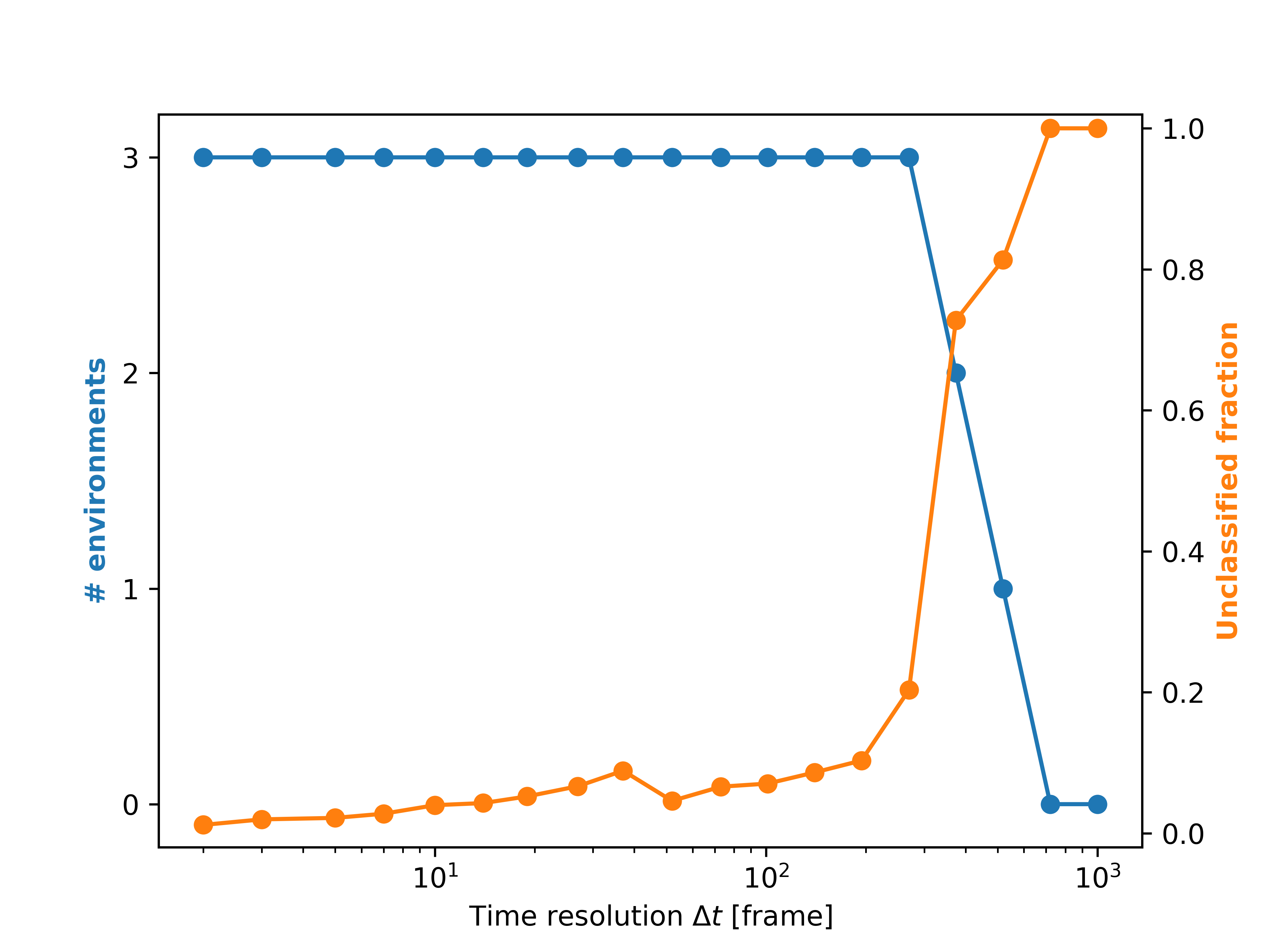
On the left are reported the results from Onion clustering on the denoised time-series (denoised_onion_analysis.png from spatial denoising tutorial), while on the rigth is reported the figure cleaned_onion_analysis.png.

Full scripts and input files

⬇️ Download the .gro file
⬇️ Download the .xtc file
⬇️ Download Python Script