Getting Started
Welcome to the first tutorial of the dynsight platform.
Before start, we strongly suggest to read the dynsight workflow page where the typical
workflow of a typical dynsight usage is described. Briefly, the reccomended way to use dynsight is via loading a trajectory into a trajectory.Trj
object, and then using the methods of this class to compute the desired descriptors and/or analyses.
In this tutorial, we will show you a minimal example of a dynsight analysis workflow;
starting from loading a trajectory, computing a descriptor and finishing
with clustering analysis.
At the end of this tutorial, you will find links to download the full python scripts
and its relevant input files.
1. Loading a trajectory
The dynsight.trajectory module provides a unified set of tools that
streamline the analysis of many-body trajectories, offering a consistent and
user-friendly interface across most analysis tasks.
This is achieved through the class, trajectory.Trj, which corresponds to an
object that contains a trajectory, meaning the coordinates of a set of particles over a series of frames.
The first step is usually to create a trajectory.Trj object from
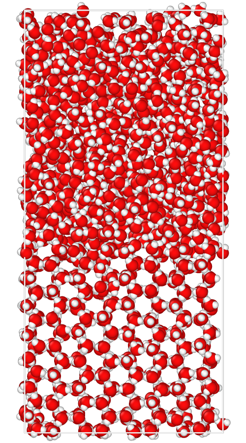
some trajectory file (e.g., .xtc and .gro files for GROMACS simulation output). In this example, we are using the water/ice
coexistence trajectory, which can be downloaded here:
 ⬇️ Download the .gro file
 ⬇️ Download the .xtc file
We now can load the trajectory using the trajectory.Trj.init_from_xtc() method. All file operations
(checking existence, opening, saving, defining a path) are done using the pathlib library.
from pathlib import Path
from dynsight.trajectory import Trj

files_path = Path("source/_static/simulations")
trj = Trj.init_from_xtc(
    traj_file=files_path / "ice_water_ox.xtc",
    topo_file=files_path / "ice_water_ox.gro",
)
Other methods to load trajectories are listed here and can be simply replaced with your format (If you need another format, please submit an issue here).
2. Computing a descriptor (the LENS case)
Now the trj variable contains the trajectory, and using the methods of the
trajectory.Trj class we can perform all the dynsight analyses on
this trajectory. For instance, let’s say we want to compute the LENS
descriptor (Crippa et al.).
This can be easily done using the trajectory.Trj.get_lens() method after the trajectory loading:
# Adjust n_jobs according to your computer capabilities
lens = trj.get_lens(
    r_cut=10,
    n_jobs=4
)
Important
The units for the r_cut parameter are the same as those used in the trajectory (In this case Angstroms).
The method trajectory.Trj.get_lens() returns a
trajectory.Insight object (lens), which in its .dataset attribute
contains the LENS values computed on the trj trajectory. Moreover, its
.meta attribute stores all the parameters relevant to this descriptor
computation, in this case:
print(lens.meta)
outputs:
{'name': 'lens', 'r_cut': 10, 'delay': 1, 'centers': 'all', 'selection': 'all'}
3. Clustering analysis using Onion Clustering
The trajectory.Insight objects can directly be used to perform post-processing such as smoothing (see the other tutorials pages).
But they can also be used to perform clustering analysis. In this example, we will show how to use the
Onion Clustering method (Becchi et al.) to cluster the LENS values computed above.
We can perform clustering on the lens object, using for
instance the Insight.get_onion_smooth() method with a time window of 10 frames:
lens_onion = lens.get_onion_smooth(delta_t=10)
lens_onion is a trajectory.OnionSmoothInsight object,
which stores the clustering output (similarly to a normal Insight object), and offers several methods to visualize
the results. Here we show some examples of visualization:
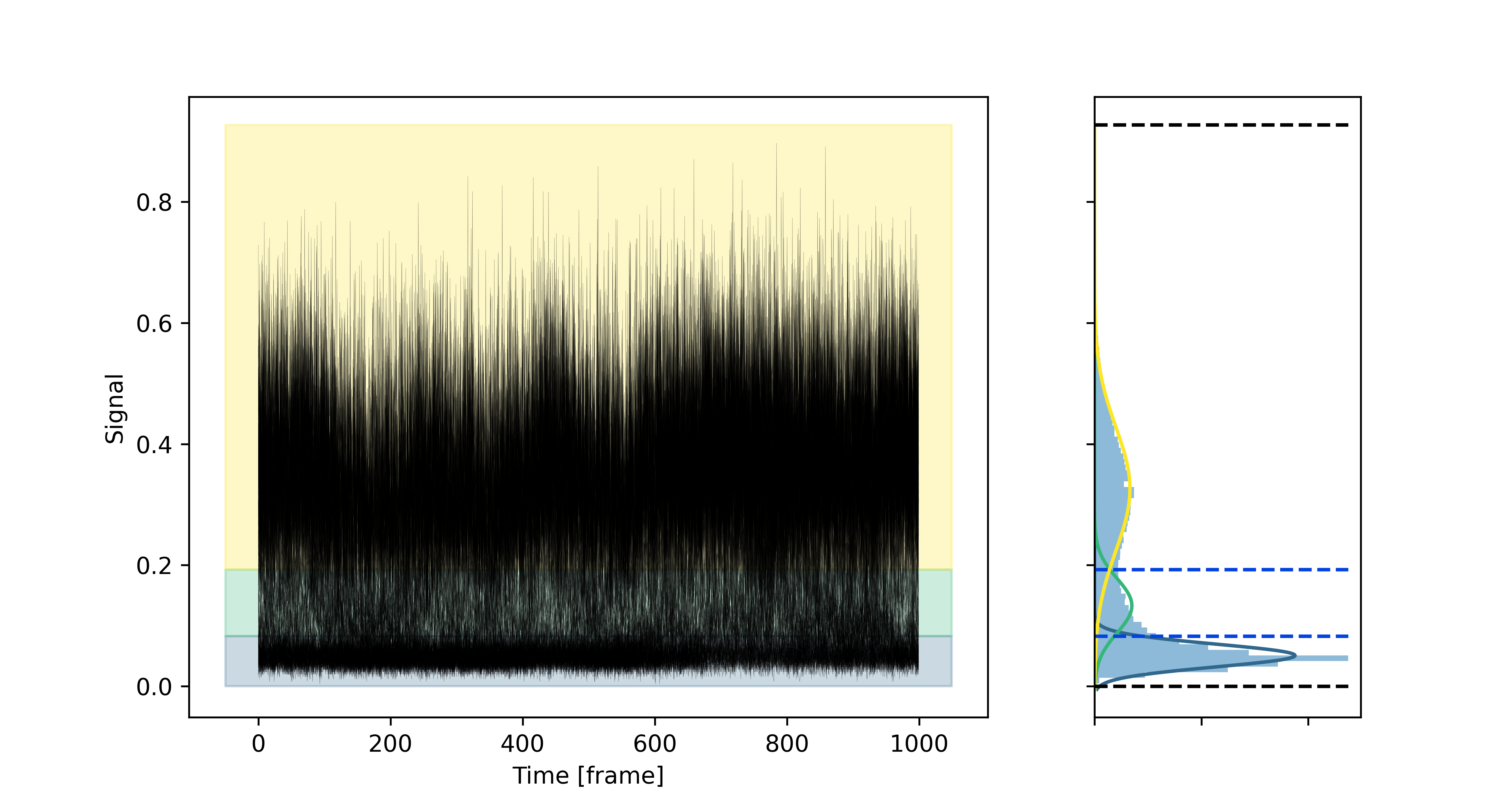
lens_onion.plot_output(
file_path=files_path / "output_plot.png",
data_insight=lens,
)
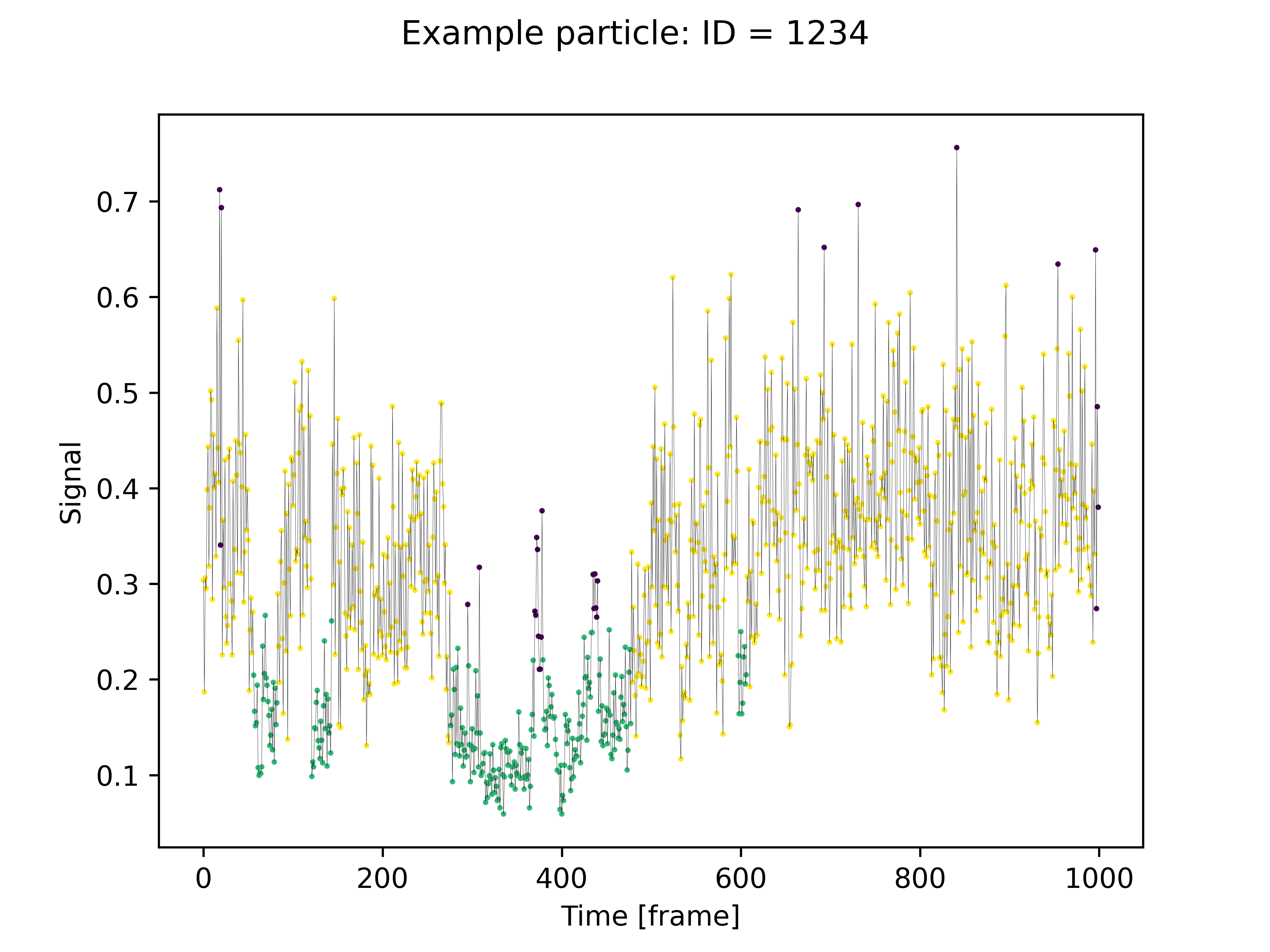
lens_onion.plot_one_trj(
file_path=files_path / "single_trj.png",
data_insight=lens,
particle_id=1234,
)
The output plot:
The single particle trajectory plot:
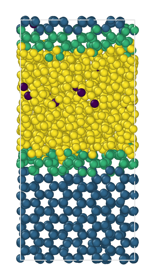
It is also possible to save a copy of the trajectory where each particle is labeled
according to its cluster assignment, using the dump_colored_trj() method. Notice that,
differently from other descriptors, which are computed for every frame, LENS
is computed for every pair of frames. Thus, the LENS dataset has shape
(n_particles, n_frames - 1). Consequently, if you need to match the LENS
values with the particles along the trajectory, you will need to use a sliced
trajectory (removing the last frame). The easiest way to do this is:
trajslice = slice(0, -1, 1)
sliced_trj = trj.with_slice(trajslice=trajslice)
Then we can dump the colored trajectory:
lens_onion.dump_colored_trj(
    trj=sliced_trj,
    file_path=files_path / "colored_trj.xyz",
)
This allows to create visualizations of the clustering results using external software such as VMD or Ovito:
Full scripts and input files
⬇️ Download the .gro file⬇️ Download the .xtc file
⬇️ Download Python Script